Home Lab 1 Lab 2 Lab 3 Lab 4 Lab 5 Lab 6 Lab 7 Lab 8 Lab 9 Lab 10 Lab 11 Lab 12 Lab 13

Lab 9

Scanning the Room

To begin this lab I developed and implemented a method to rotate the car as slowly as I could around a point. I chose to do this using angular speed control and what essentially ended up being just an integral controller. To do the control, I first passed in a target angular speed at which I wanted my car to rotate at over bluetooth. I then looked at the gyroscope value of the car and compared it to the target angular velocity. I subtracted the two and added this to a term which I then scaled and set as the PWM for the motor. This is summarized below.

turnrate=0;
while angle<360:
  error=desiredAngularVelocity-measuredAngularVelocity;
  turnRate+=I*error; //adjust the turnrate
  turnCar(turnRate); //adjust the pwm according to the turnrate
  angle+=dt*measuredAngularVelocity;
  if carIsTurningFastEnough:
    take and log a TOF measurement

In effect this led to the car staying still for a bit while it “accumulated enough PWM” to begin moving, but once it began moving, it moved very slowly and fairly smoothly which was the goal as it allowed me to take a lot of distance measurements over the course of one rotation. I did not want to have a ton of measurements where the car was just standing still because it was still building up enough power to start turning, so I implemented a check to only take a measurement when the measured PWM was a certain percentage of the desired PWM. The result of my implementation is shown in the videos below.

Below is a graph that shows the PWM over time for a given run. You can see that the PWM ramps and then oscilates around a target as expected.

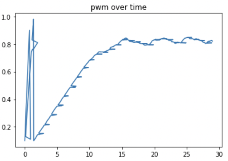
I set my target speed to 20 degrees per second which seemed to work fairly well. If you look at the video above it takes about 20 seconds for my robot to complete one turn which means I am turning at about 20 degrees per second which again was my target. I would be interested to see how low I could push the target degrees per second for my controller and have it still work. I would likely have to increase the integral coefficient term which would likely increase the oscialltion at the top and might make the turn less smooth. Nonetheless, I think that this graph, analysis, and video demonstrate my contoller works sufficiently well which is confirmed when I used it to actually start mapping.

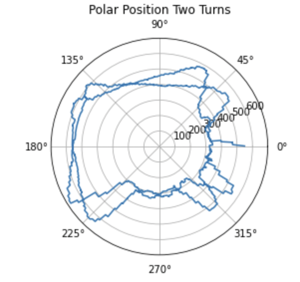
Over multiple turns the the TOF readings seem to be failry precise, but the error in the integrated angle grows more and more. The plot below shows the data over 2 consecutive turns. You see that the shap of the curves are very similar, but that the corresponding point from one turn to another appears to be rotated by a significant amount which supports my statement above.

Given the slowest speed you are able to achieve, how much does the orientation of the robot change during a single measurement? If you were spinning in the middle of a 4x4m2 empty, square room, what kind of accuracy can you expect?
By looking at the number of ToF readings I had and the total time of my run, it seems that I was getting about 6 ToF readings per second from my front ToF sensor which seems reasonable. As previously mentioned, I was turning about 20 degrees per second which means that each one of my ToF readings spanned about 20/6 or 3.33 degrees on average. From observing my robot, it seems that the center drifted by no more than about 6 inches during a given turn. 6 inches is 152.4 mm which I believe is more significant than the typical amount of error solely from sensor noise and innacuracies assuming your sensors are measuring what they are intened to. I will assume the max error you would achieve is 200 mm off because I feel that it is better to overestimate your error than to underestimate it in most cases. If you were rotating in 4mx4m room, this would mean that you would have a percent error of 5% which I got by getting .2m divided by 4m times 100 percent.

After I had the robot turning slowly, I desgined a debugger that allowed me to send information over from the car to my computer for the turn. In addition to my original log, I also sent over a log that consisted of packets with the angle as well as the front TOF reading and the side TOF reading at that angle at some point during the turn. I cacluated the angle by integrating the gyrocsope value over my loop. I adjusted my handler function so that it also filled out this “turn log” (on the Python side) in addition to the main log that I have been using throughout the class. The modified handler function is shown below. This code exploits the fact that the turn log entries are a differnt length than the main log entries. Also now is a good time to mention that I only ended up using the front TOF readings because the side sensor readings seemed to be faulty. I think that it might have been picking up on the wheel of my robot which I could fix by adjusting the positioning of the sensor, but by the time I realized this, it was not worth the effort to go back and redo the scans as I got a pretty solid map with just the front TOF as you will see below.

def updateValue(uuid,value):
    global log
    global turnLog
    received=value.decode('utf-8').split(',')
    if len(received)==3:
        turnLog.append(received)
    else:
        log.append(received)

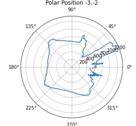
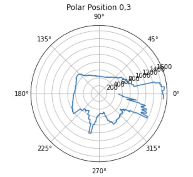
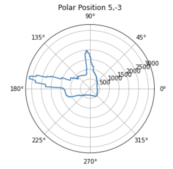
Once I had this information on my laptop, I was able to plot it in polar format and then convert that to cartesian format for each point. I then translated these plots to the reference frame of the actual origin on the map so that they could be combined later on. These plots are shown below.

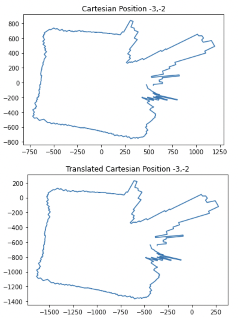
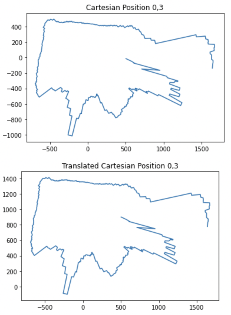
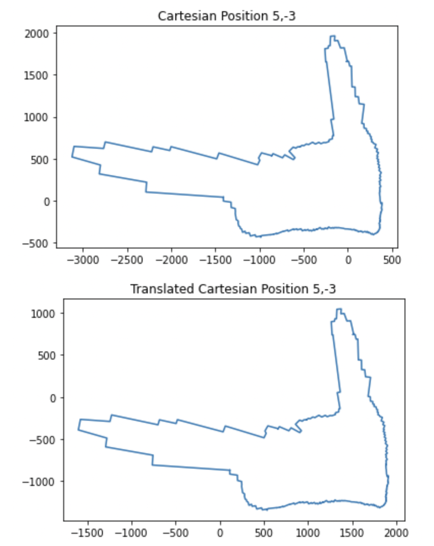
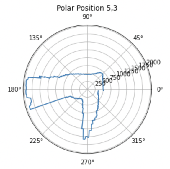
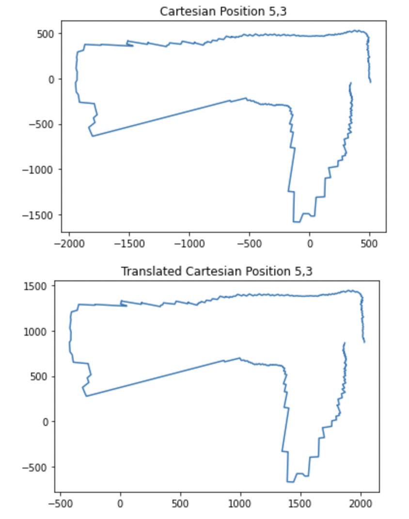
In order to translate the plots from the reference of where the turn occured to the reference frame of the origin, all I had to do was add the x value of the point where it was taken to all of the x values of the points in that rotation and the y value of the point where it was taken to all of the y values of the points in that rotation. For example if I was translating the scan from point 3,5 to the origin, I just added 3 to all of the x values and 5 to all of the y values in the cartesian map gerneated at that point. An example of the code I used to do this for one of the points is below. I also negated the theta value because I took the absolute value of it on the robot before passing it over and I was turning clockwise.

info=dataFromTurn
theta=[]
front=[]
side=[]
for i in info:
    theta.append(-1*float(i[0]))
    front.append(float(i[1]))
    side.append(float(i[2]))
for i in range(len(theta)):
    theta[i]=theta[i]*math.pi/180
# sideTheta=[]
# for i in theta:
#     sideTheta.append(i-math.pi/2)

plt.polar(theta,front)
plt.title("Polar Position 0,3")
plt.show()

x=[]
y=[]
for i in range(len(theta)):
    x.append(front[i]*math.cos(theta[i]))
    y.append(front[i]*math.sin(theta[i]))
plt.figure("catestian")
plt.title("Cartesian Position 0,3")
plt.plot(x,y)

xcorrected1=[]
ycorrected1=[]
for i in x:
    xcorrected1.append(i)
for i in y:
    ycorrected1.append(i+914.4)
plt.figure("catestian translated")
plt.title("Translated Cartesian Position 0,3")
plt.plot(xcorrected1,ycorrected1)

The easy switch from one reference frame to another was made possible by the fact that I started my robot pointing towards 0 degrees (in the positive x direction) before every scan. Thus no rotational transformation was required only translational and I avoided needing transformation matrices as they only complicated things.
I then plotted the transformed maps all on the same plot and this was the final result of my mapping.
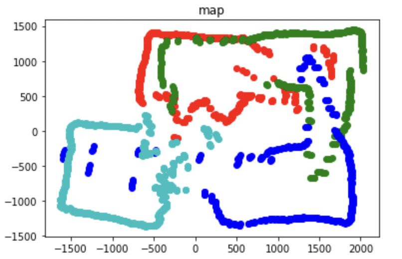
This map is decent. There ae some spots where it could definitely be improved. The I smashed my robot’s TOF sensor in the last lab, and when I remounted a new one, it seemed like it was pointing up slightly. This was not a problem for measuring the walls that were close, but I believe it might have overshot some of the walls that were farther away, as the walls were not very high, causing some erroneous measurements. This is shown in the image below.

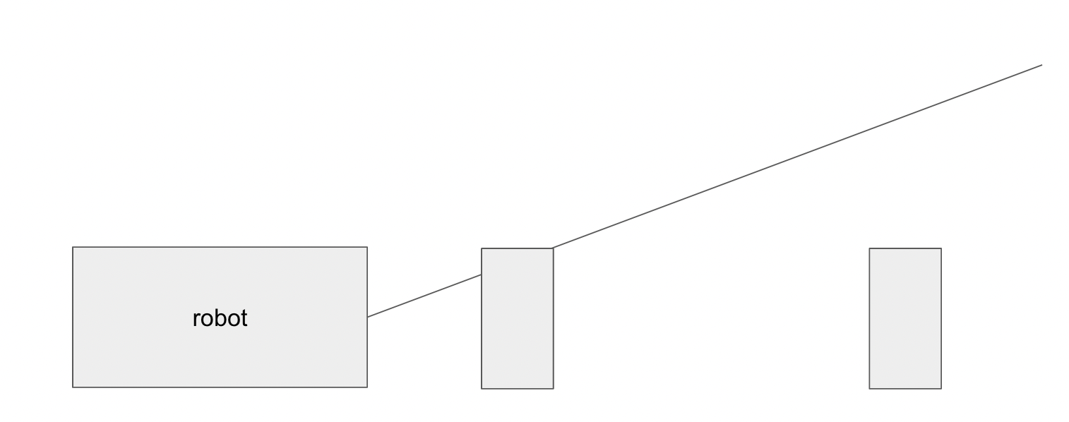
In addition there will always be some noise in the sensors and my robot did not turn perfectly around the point that it was rotating on as you saw in the videos above.
Below is the line based version of the map that I generated based on my plot. I corrected for some of the erroneous readings by using the parts of the plot map that seemed very accurate in tandem with my previous experience with the layout of the arena.

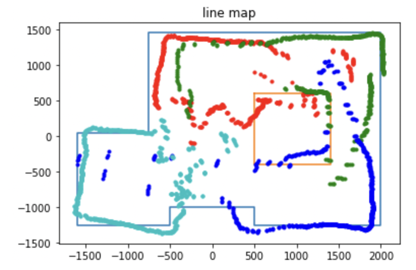
The code below shows the points I used to genrate this map. I am putting this here for reference and for ease of access when I need it in the next lab.

# line based map
start=[]
end=[]
boxstart=[]
boxend=[]
start.append((-750,1450))
end.append((-750,50))
start.append((-750,50))
end.append((-1600,50))
start.append((-1600,50))
end.append((-1600,-1250))
start.append((-1600,-1250))
end.append((-500,-1250))
start.append((-500,-1250))
end.append((-500,-1000))
start.append((-500,-1000))
end.append((500,-1000))
start.append((500,-1000))
end.append((500,-1250))
start.append((500,-1250))
end.append((2000,-1250))
start.append((2000,-1250))
end.append((2000,1450))
start.append((2000,1450))
end.append((-750,1450))

boxstart.append((1400,600))
boxend.append((500,600))
boxstart.append((500,600))
boxend.append((500,-400))
boxstart.append((500,-400))
boxend.append((1400,-400))
boxstart.append((1400,-400))
boxend.append((1400,600))

x=[]
y=[]
boxx=[]
boxy=[]
end.append(start[1])
boxend.append(boxstart[1])
for i in end:
    x.append(i[0])
    y.append(i[1])
for i in boxend:
    boxx.append(i[0])
    boxy.append(i[1])
plt.title('line map')
plt.plot(x,y)
plt.plot(boxx,boxy)
plt.plot(xcorrected1,ycorrected1,linestyle="",marker=".",color='r')
plt.plot(xcorrected2,ycorrected2,linestyle="",marker=".",color='g')
plt.plot(xcorrected3,ycorrected3,linestyle="",marker=".",color='b')
plt.plot(xcorrected4,ycorrected4,linestyle="",marker=".",color='c')