Lab 8
Do Not Hit The Wall!
To start, this lab I thought about which pieces of the old labs I could incorporate into my solution. I decided that the Kalman filter would be the only thing that I would need. I wanted to sample from my Kalman filter as fast as possible, and I sped up my sampling rate in two ways. First I divided up my Kalman filter into two stages, the prediction stage and the update stage. The prediction stage was run every time through the loop in my code. The update stage was run only when there was a new front TOF sensor value that the Kalman filter had not seen. In this way I could sample my Kalman filter much more quickly than I could sample my TOF sensor and thus could make predictions about where I was and update my state variable while waiting for a new sensor value. I accomplished this with a kfReady variable. When the TOF sensor read a new variable, it would set kfReady causing the KF to perform the update step on the next pass through. When the KF had performed the update step it set kfReady back to 0 indicating the KF had been updated by the most recent TOF reading. The code for the updated KF is shown below.
Matrix<2,1> state = {0,0};
Matrix<1> u = 0.0;
float drag=.001;
float m=.0009988773;
Matrix<2,2> A = {0,1,
                 0,-1*drag/m};
Matrix<2,1> B = {0,1/m};

Matrix<1,2> C = {-1,0};
//Matrix<1> sig_z=20.0; ///lower to trust sensor values more
//Matrix<2,2> sig_u = {25,0,
//                     0,50};  ////lower these and the sig z to make kalman filter more aggressive ie lag less

Matrix<1> sig_z=10.0; ///lower to trust sensor values more
Matrix<2,2> sig_u = {15,0,
                     0,35};  ////lower these and the sig z to make kalman filter more aggressive ie lag less

Matrix<2,2> sig = {25,0,
                   0,25};
///delta_t computed on previous data
Matrix<2,2> Ad = {1,.0092,
                  0,.991};
Matrix<2,1> Bd = {0,9.24704833};

//values to alter
Matrix<2,1> xn;
Matrix<2,2> sign;

void kf(Matrix<2,2> sigma, Matrix<1> frontSensorValue){
  if (kfReady==1){  //run prediction and update step
    Matrix<2,1> xp=Ad*state+Bd*u;
    Matrix<2,2> sigp=Ad*sigma*~Ad + sig_u;
    Matrix<1> ym=frontSensorValue-C*xp;
    Matrix<1> sigm=C*sigp*~C+sig_z;
    Invert(sigm);
    Matrix<2,1> k_gain=sigp*~C*sigm;
    xn=xp+k_gain*ym;
    Matrix<2,2> I={1,0,
                   0,1};
    sign=I-k_gain*C*sigp;
    sig=sign;
    state=xn;
    kfReady=0;  ///kalman filter has seen the most recet data
  } else {  //run only the prediction step
    Matrix<2,1> xp=Ad*state+Bd*u;
    Matrix<2,2> sigp=Ad*sigma*~Ad + sig_u;
    sig=sigp;
    state=xp;
  }
}
The other way in which I sped up my kf sampling rate, was that I removed any code where I sampled from the side TOF and the IMU. This information was not useful in this lab and thus I did not waste time collecting it.
At this point I was able to update my state variable extremely quickly. Again this is important becuase I am using my state variable to determine when I needed to flip. I then began updating my code to perform a flip. I wrote code that drove the car in one direction until the state(0,0), the predicted position of the car, was sufficiently small, and then I drove it back in the other direction. I started slow which is shown in the video below.
My main loop that I used to accomplish this is shown below.
startTime=millis();
while (central.connected()) {
    timeStamp=millis();
    updateSuccess=myBot.updatePosition(); //grab new TOF sensor reading if available and the is a new reading set kfReady
    while (myBot.front==0) myBot.updatePosition(); //accounts for the 0s it reads at the beginning of the run
    kf(sig,myBot.front); //sample the kalman filter
   ///if I get close enough to the wall go the other way
    if (-1*state(0,0)<=int(p) && -1*state(0,0)!=0 ) dir=-1;
    myBot.forward(dir,-1*state(0,0),-1*state(1,0)); //pass in kalman filters for bot to log
    u=dir; //update u matrix
    logSuccess=myBot.logIt(timeStamp-startTime);  //log sensor information and KF information
    if (logSuccess==0){ ///if the log is full end the run and stop the robot
      break;
  }
}
myBot.STOP();
Now that I was getting through this loop much more quickly than in Lab 7 and sampling my KF everytime through, I needed to adjust the discretized A and B matrices. In order to adjust them properly, I collected data on one run with my bot. I then used Python to average the time it took to get through each loop and used that as my new delta_t when descritizing the original A and B matrices that I found in lab 7. The way I computed the new Ad and Bd are shown below.
### got a new log for faster code with only front TOF sensor running
###lab 8 recalculating descritized A and B matrices
s=0
for i in range(len(log)-1):
    s+=(float(log[i+1][0])-float(log[i][0]))
avg=s/len(log)
print("average is " +str(avg) + " seconds")
delta_t=avg

d=.001
m=.0009988773
A=np.array([[0,1],[0,-1*d/m]])
B=np.array([[0],[1/m]])
### discretize A and B
Ad=np.eye(2)+delta_t*A
Bd=delta_t*B
If you look in the KF code above on the Artemis, you can see that Ad and Bd have been updated accordingly.
Despite driving at a significantly different max speed I figured that I did not need to adjust my non-descritized A and B matrices. I thought that since d was the step reponse divided by the velocity and becuase the velocity scales with the step response, d would be approximately equal for a higher PWM value/top speed. Additionally, m is calculated as d times the 90% rise time divided by ln(.1). I figured that the original 90% rise time would be similar to the 90% rise time of my new step input with a bigger max PWM the car will accelerate faster, but will also need to increase its speed more to reach its’ “top speed” as this grows with a higher PWM value as well. Because of this I did not update the d and m values when going to a higher speed and thus did not need new non-descritized A and B matrices. Additionally a “u” term of 1 still represented top speed regardless of what that speed was. My implementation ultimately worked well so this seemed to be reasonable. Perhaps these assumptions would have affected me more had I set my sigma values to place more trust in my model.
Once I had this working, it was really about tuning the robot. There were 4 parameters that I needed to tune, run length, speed towards the wall, reverse speed, and distance at which the bot reverses.
In my code, my bot runs until it fills up its log and then it stops. Becuase I was going through my loop so much faster and thus making entries into the information log much more frequently, I needed to play around with the log length until it caused the bot to run for an appropriate amount of time. If it was too short, it died before it fully executed the maneuver. If it was too long, the bot would likely crash into something going full speed.
When adjusting the speed at which the bot approached the wall and drove away from the wall, I started slow and worked my way up. However, I soon learned that in order to get the car to flip, I would need to drive towards the wall very quickly and then reverse at full speed when I hit the mat. At this point it mostly became about tuning the distance at which the car started reversing. If you started it too soon, by the time the car got onto the mat, it would be going too slow to flip. If you started it too late, the car would likely overshoot the mat and hit the wall. I discovered the I needed to start reversing about 1100 mm away from the wall. This yielded good results and I was able to successfully and quickly complete my flip and return past the starting line as the video shows.
The bot flips and quickly travels back past the starting line. However, when it flips, it does so at a slight angle which is my only complaint with the performance of my solution. I could have tried to find a different proportion at which to drive the motors during the flip in order to accomplish a more even flip. The final proportion was I drove the right motor at a PWM of 245/255 and the left motor at a PWM of 255/255. Again, adjusting these values might help the bot flip more evenly.
In addition to tuning, Anya (who was in the lab with me when I was testing) and I found some additional ways in which we could help our robots flip. We found that it helped to clean the robots wheels as well as the sticky mat which accumulated dust quite quickly. Additionally, we found that it was important to replace the battery pretty frequently to ensure maximum velocities needed for the car to flip.
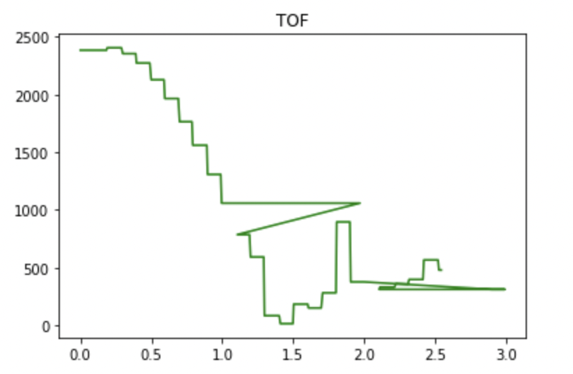
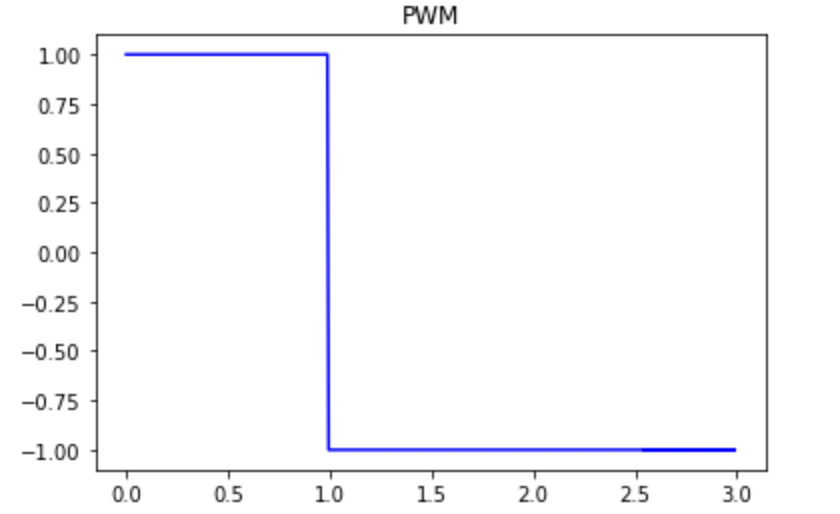
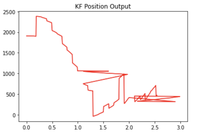
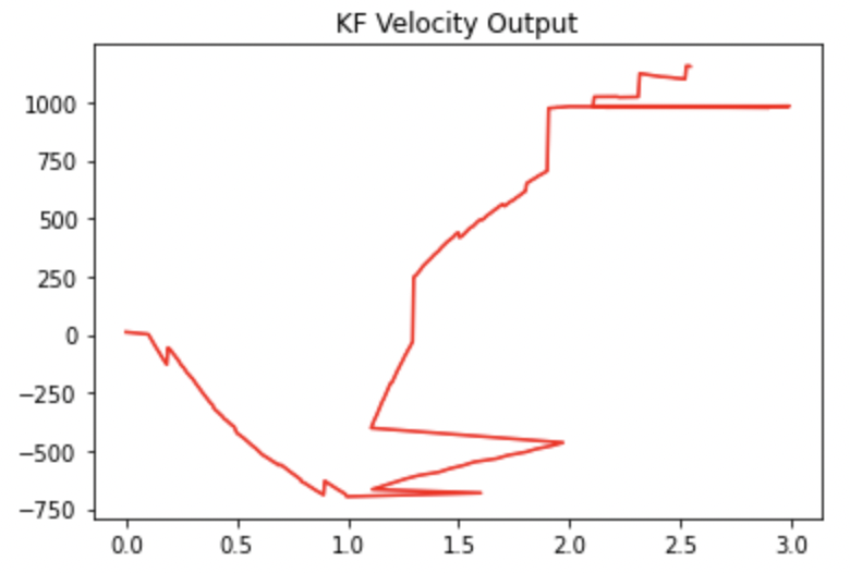
Below are the requested graphs of the data taken from a run with a successful flip. The TOF output is shown. The ouput of the Kalman filter is shown in two separate graphs, one for the position prediction and one for the velocity prediction. Notice how the Kalman filter position prediction is smoother (it lacks the “steps” at the beginning) indicating that it is making predictions and updating its predicted state even between successive TOF readings which was a major goal for the KF (because I am running the prediction step every time through the loop). The KF velocity graph shows an increasing velocity, but the velocity increases by less and less (concave down) as the car approached the wall. The PWM signal is either full speed ahead, 1, or full speed backwards, -1. The TOF readings and KF outputs are nonsense after the robot flips as one would expect. One can see that the flip happened about 1 second into the run and this lines up nicely in all of the graphs giving us more confidence that it is indeed good data.
In the end the Kalman Filter helped me account for slow TOF sensor readings and update my state much more quickly via the prediction step allowing me to flip at the right time and successfully perform the stunt!
Open Loop 720
For my open loop stunt I performed what I term a 720 spin-out. Essentially the car goes forward, drifts one way, and then turns sharply the other way causing it to spin out. I hold the spin-out for 2 loops around and then drive the car forward back in roughly the original direction. Below is the commented control sequence I used to accomplish this as well as 3 videos showing the stunt and demonstrating its repeatability.
analogWrite(3,255); //// go straight
analogWrite(16,255);
delay(1000);
analogWrite(1,0);
analogWrite(3,255);

analogWrite(14,100); //turn a bit
analogWrite(16,0);
delay(500);
analogWrite(14,0);
analogWrite(16,80); //turn back the other way initiating spin out
delay(1000);

analogWrite(1,0);
analogWrite(3,255); ///drive forward

analogWrite(14,0);
analogWrite(16,255);
delay(3000);
analogWrite(1,0); //stop
analogWrite(3,0);

analogWrite(14,0);
analogWrite(16,0);
Bloopers