Home Lab 1 Lab 2 Lab 3 Lab 4 Lab 5 Lab 6 Lab 7 Lab 8 Lab 9 Lab 10 Lab 11 Lab 12 Lab 13

Lab 7

1. Step Response

In lab 6, I drove one of my motors at a PWM value of 65/255 and the other at a PWM value of 55/255. Because of this I drove the car at the wall with the crash pad using the same PWM values (without PID) and recorded the run so that I could analyze the step response. The way I designed my bot, I am easily able to change the timing of the run. I played around with this time and found a run length that would get it up approximately to full speed for a given PWM value and would stop right after that so that it did not hit the wall too fast.
My data is recorded in entries and is sent over to my computer. However, my TOF code is non-blocking and the IMU runs much faster than the TOF sensors, thus multiple log entries often contain the same TOF sensor reading. Becuase of this, I filtered out data log entries with repeat front TOF sensor readings.
I eventually came up with the following data.

Motor Step Response

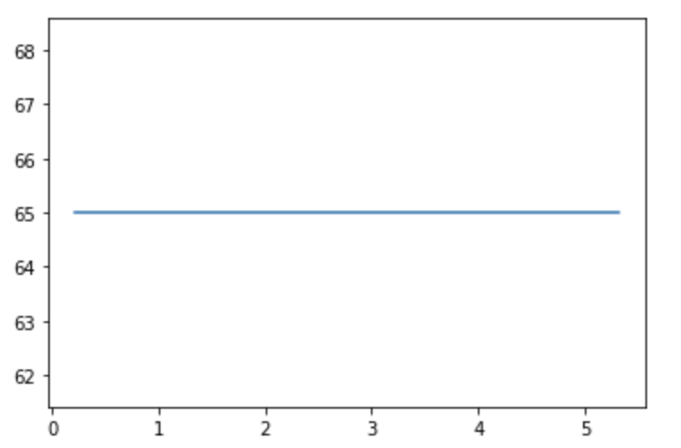
TOF Sensor Readings

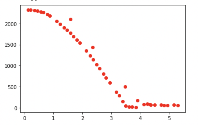
Calculated Speed

To generate the speed graph, I looked at successive TOF sensor readings, found the distance between them, and then divided by the time between the readings.
By looking at the speed graph I can see that it looks like my robot gets up to about 1.1 m/s and it took it about 2.3 seconds to rise to 90% of this value. It would have been better to let the robot run a little bit longer and see the curve flatten out to a more constant speed, but the curve is defintitely starting to flatten out and I did not want to crash my robot into a wall.
Using this information allowed me to compute my A and B matrices. Using d=u/v where I am using 1 as u to represent the unity step response, and v is velocity, I can see that steady state drag, d, is 1/1000mm/s or d=.001
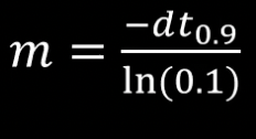
Then using the equation in the image shown below and the 90 percent rise time of 2.3 seconds to calculate m,, I get m=.0009988773

2. Kalman Filter Setup

In this section I specify process noise and sensor noise. Sensor noise as the name suggests depends on my sensor. In lab 2 I wrote some code that took a bunch of TOF sensor readings off of the front sensor and outputed the variance of the measurements. I saw that the variance seeemed to increase when the sensor was measuring a longer distance which seems to intuitevly make sense. I saw that at a distance around 100 mm that variance seemed to be about 12 mm^2. Because my robot will often be taking measurements much farther out than this, I will make the sensor noise much bigger. I will assume sensor noise/ variance of 25 mm^2. This seems reasonable and is similar to the sensor noise value of 20 mm^2 assumed by Professor Peterson in lecture which is reassuring.
In order to determine process noise, I tried to reason about how far off my Kalman filter would be everytime it was run and also how many times it would be run. By analyzing my TOF sensor data sent over after my run, it looks like I am updating a TOF value about 10 times per second. It also makes sense that I will only run my Kalman filter when I have a new measurement to feed into it, so I will run my Kalman filter about 10 times per second as well. In class Professor Peterson estimated that her robot position prediction would be off about by about 5 mm and her robot velocity prediction would be off by about 10 mm/s everytime through the Kalman filter which she was running about 50 times per second. These estimates seem somewhere in the realm of reasonable (i.e. they are not 100 m every second) and they seemed to provide her with solid results in class. Additionally, we are operating very similar robots in very similar conditions, so I figure that I should be able to use similar process noise values in my lab. However, as I mentioned she was assuming a sampling rate of 50 times per second where I am at 10 times per second so I am going to multiply her values for error everytime through the filter by 5. Explained simply, the more time in between samples of my Kalman filter the more error will accumulate between samples. Thus everytime I sample my Kalman filter I am assuming my predicted position process noise is 25 mm and my predicted velocity process noise is 50 mm.

sig_u=np.array([[25,0],[0,50]]) ### process noise (assumed process noise every time I sample the Kalman filter)
sig_z=np.array([[25]]) ### measurement noise (variance of sensor)

My C matrix is a m by n matrix where n is the number of dimensions in my state space and m is the number of states I actually measure. There are 2 dimensions in my state space x and v and I actually only measure x so my C matrix looks like

C=np.array([[-1,0]])

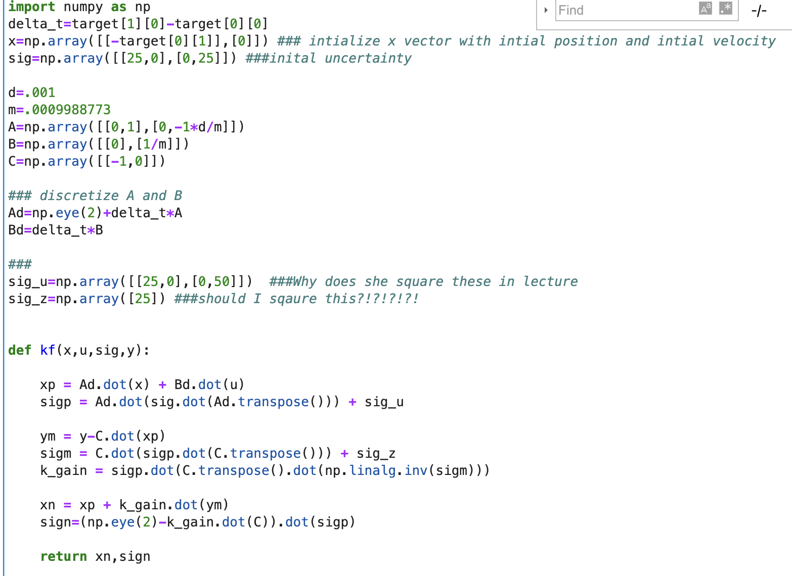
3. Sanity Check Kalman Filter

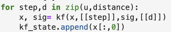
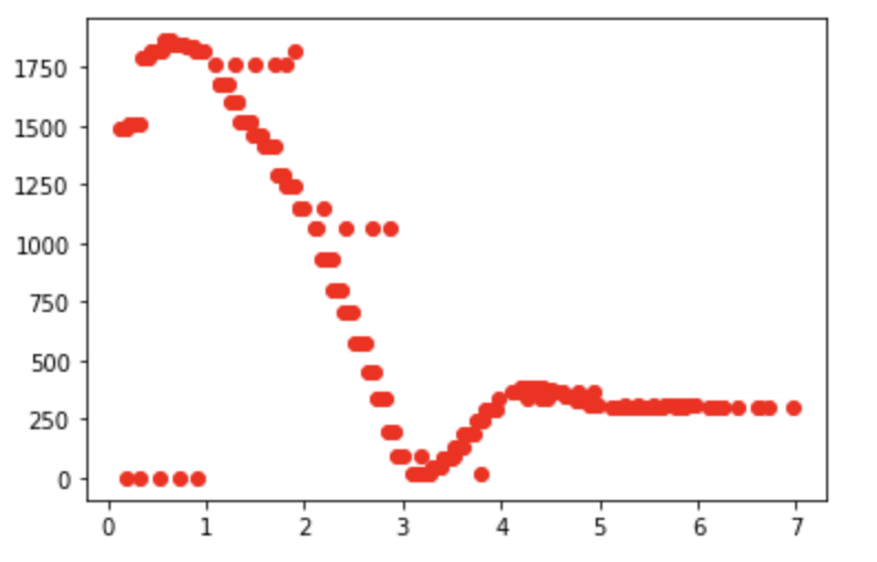
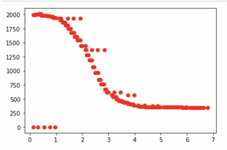
In order to sanity check my Kalman filter I used Python. I created numpy arrays for my A, B, and C matrices filling in the values that I discussed above. I then referenced the provided code and in class tutorial to create a Kalman filter function. Loading in my data from lab 6 I then compared the actual TOF sensor readings with the output of my Kalman filter and compared the results. The screenshots below show the important pieces of my Python code. As is evident in the code the red line is the Kalman Filter and the Blue line is the TOF sensor.




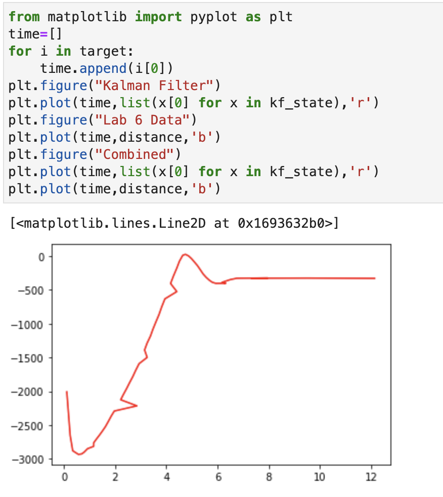
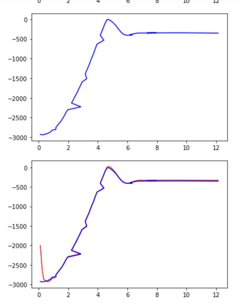
As you can see the Kalman Filter appears to be working as it follows the TOF sensor fairly closely. This gave me confidence to move it over to the robot.
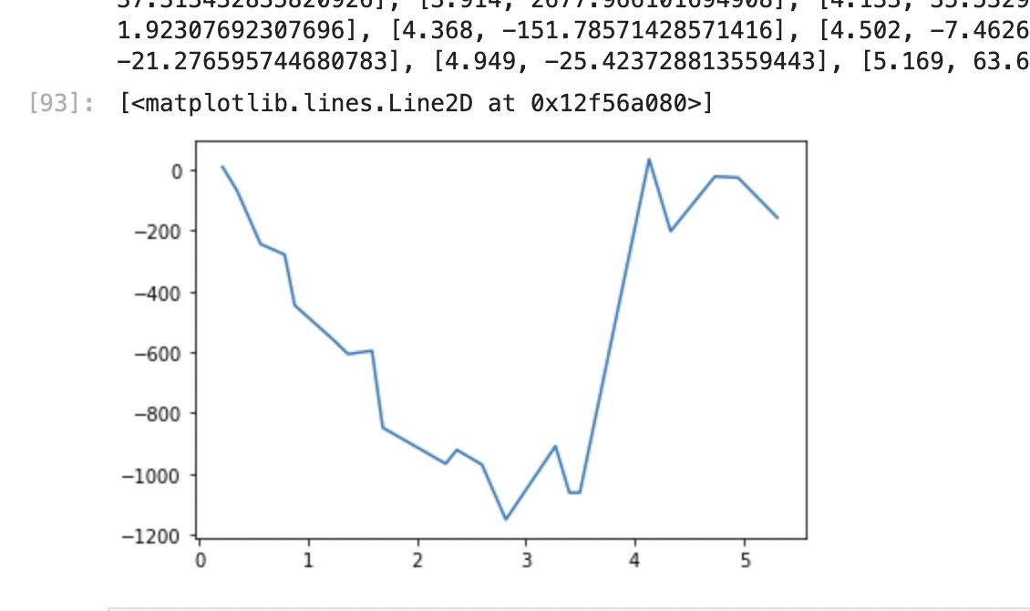
In addition to the graph of the TOF sensor readings, one might find the graph of the motor output interesting as well and thus it is shown below.

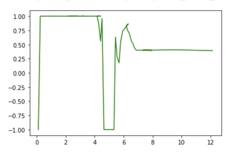
These graphs are alittle bit strange because there are some points where it is not a function. I suspect that this is due to a small error in my filtering out log entries without updated TOF sensor values. However, the overall shape of the graph makes a lot of sense and this slight error is of minimal concern.

4. Kalman Filter on the robot

I then took the kalman filter (KF) Python code and implemented it on my robot. This “translation” is shown below.

Matrix<2,1> state = {0,0};
Matrix<1> u = 0.0;
float drag=.001;
float m=.0009988773;
Matrix<2,2> A = {0,1,
                 0,-1*drag/m};
Matrix<2,1> B = {0,1/m};

Matrix<1,2> C = {-1,0};

Matrix<1> sig_z=10.0; ///lower to trust sensor values more
Matrix<2,2> sig_u = {15,0,
                     0,35};  ////lower these and the sig z to make kalman filter more aggressive ie lag less
                     
Matrix<2,2> sig = {25,0,
                   0,25};
///delta_t computed on previous data
Matrix<2,2> Ad = {1,.132,
                  0,.86785164};
Matrix<2,1> Bd = {0,132.148};

//values to alter
Matrix<2,1> xn;
Matrix<2,2> sign;

void kf(Matrix<2,2> sigma, Matrix<1> frontSensorValue){
  Matrix<2,1> xp=Ad*state+Bd*u;
  Matrix<2,2> sigp=Ad*sigma*~Ad + sig_u;
  Matrix<1> ym=frontSensorValue-C*xp;
  Matrix<1> sigm=C*sigp*~C+sig_z;
  Invert(sigm);
  Matrix<2,1> k_gain=sigp*~C*sigm;
  xn=xp+k_gain*ym;
  Matrix<2,2> I={1,0,
                 0,1};
  sign=I-k_gain*C*sigp;
  sig=sign;
  state=xn;
  kfReady=0;  ///reset this back to 0 indicating kalman filter has been run on most recent data
}

You can see in this code that I made my sigma u and sigma z values smaller than they were in the Python code. I made the sigma z value smaller, because my robot kept crashing into the wall and I thought that it needed to trust the sensor values more. I then lowered the other values to make the KF slightly more aggressive and thus slightly more responsive. I found that these values worked well as shown in the videos at the bottom.
I added in the kfReady variable to help me keep track of whether or not the KF has been run on the most recent data or not. When new data is read from the TOF sensor by the bot, it sets kfReady to 1 indicating that the KF needs to be run on those readings. Once the KF runs, it will set it back to 0 indicating it has seen the most recent TOF sensor data. In lab 8 I will likely use this kfReady to run the prediction step every time through loop and only run the update step of the KF when there is new data.

The robot then takes TOF readings, feeds them through the kalman filter (KF), and feeds the KF output into the PID controller. The jist of this code is shown below.

/// only run kalman filter if there is new sensor data to run it on (kfReady) and ignore the zeroes the TOF sensors spit out at the beginning
 if(kfReady==1 && myBot.front!=0){
            kf(sig,myBot.front);//run kalman filter which updates "state" matrix
          }
          theerror=-1*state(0,0)-300;  /// calculate the error based on kalman filter output
          
          // keep a history for the derivative term
          pe[0]=pe[1];
          pe[1]=pe[2];
          pe[2]=pe[3];
          pe[3]=-1*state(0,0);  ///by not using "theerror" here you protect against changes in the setpoint while achieving a very similar effect
          
          myBot.forward(p*float(theerror)+float(d*(pe[3]-pe[0]))); //drive the bot based on this information
          
          if (p*float(theerror)+float(d*(pe[3]-pe[0]))>1){ ///update u
              u=1;
            } else if((p*float(theerror)+float(d*(pe[3]-pe[0]))<-1){
              u=-1;
            } else{
              u=p*float(theerror)+float(d*(pe[3]-pe[0]));
            }

I also experimented with further tuning my PID controller and got some promising results which are shown in the two videos below. In the first video I have a lower D term and thus my robot approaches the wall faster, but it overshoots. In the second video, I run the robot with an increased D term and it approaches the wall more slowly, but does not overshoot. I am hoping that this improvement will serve me well in the future and help me protect my bot in lab 8.

Below you can see the TOF readings for one of the faster runs (D term is smaller). As you can see there is a greater slope in the data but more oscillation.

Below you can see the TOF readings for one of the slower runs (D term is larger). As you can see there is a more gradual slope, but minimal overshoot and oscillation.

At the end of this lab I was thinking about how I might get the robot to resist high changes in velocity only when it is near the wall. I came up with the solution of doing something to the the effect of

myBot.forward(p*float(theerror)+((A/myBot.front)**2)float(d*(pe[3]-pe[0])));

In this way when the bot approaches the wall myBot.front, the front sensor reading, will be much smaller making the term in front of the d coefficient much larger, causing the d term to affect the robot much more at distances closer to the wall and less when further away. This would hopefully let the robot experience smooth and powerful acceleration at the beginning of the run while still slowing it down when it gets close to the wall at high speeds. I did not have time to really test this, but it might be something I revisit later in the semester.