Lab 3
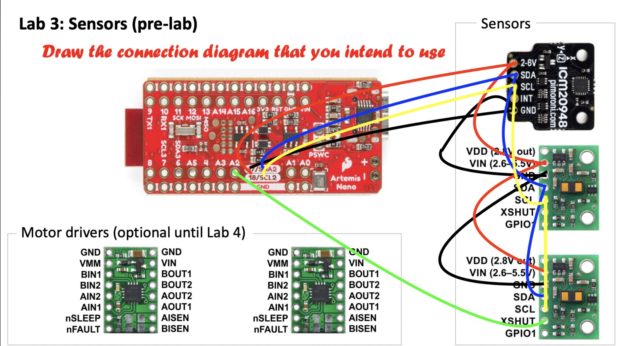
Below is my circuit diagram showing how I hooked up the three sensors so that they could communicate to the Artemis using I2C. I am choosing to set the shutdown pin one on of the TOF sensors, change the address of the other, and then re-enable the TOF sensor instead of shuting one down before every transaction. I do all of this in setup so that it is only run once. Here is the pseudo code:
declare sensor 1;
declare sensor 2;
pull shutdown pin on sensor 1 low;
change I2C address of sensor 2;
set shutdown pin on sensor 1 high; // re-enabling it
interact with sensor 1;
interact with sensor 2;
The benefit of doing it this way is that I use less wires, because I would need to have a shutdown wire going to sensor 2 if not. This implementation is also more efficient because I only need to spend time setting a shutdown pin once at the beginning and do not need to worry about it any more. Toggling between the two sensors shutting one down and reading from the other, would likely be more memory efficient as I would likely only need one sensor object in my program. I will place one TOF sensor on the front of the robot and one on the side. It seems that I might miss objects that are in between these two sensors field of views as well as on my blind side and in the back.
part 3a Time of Flight Sensors
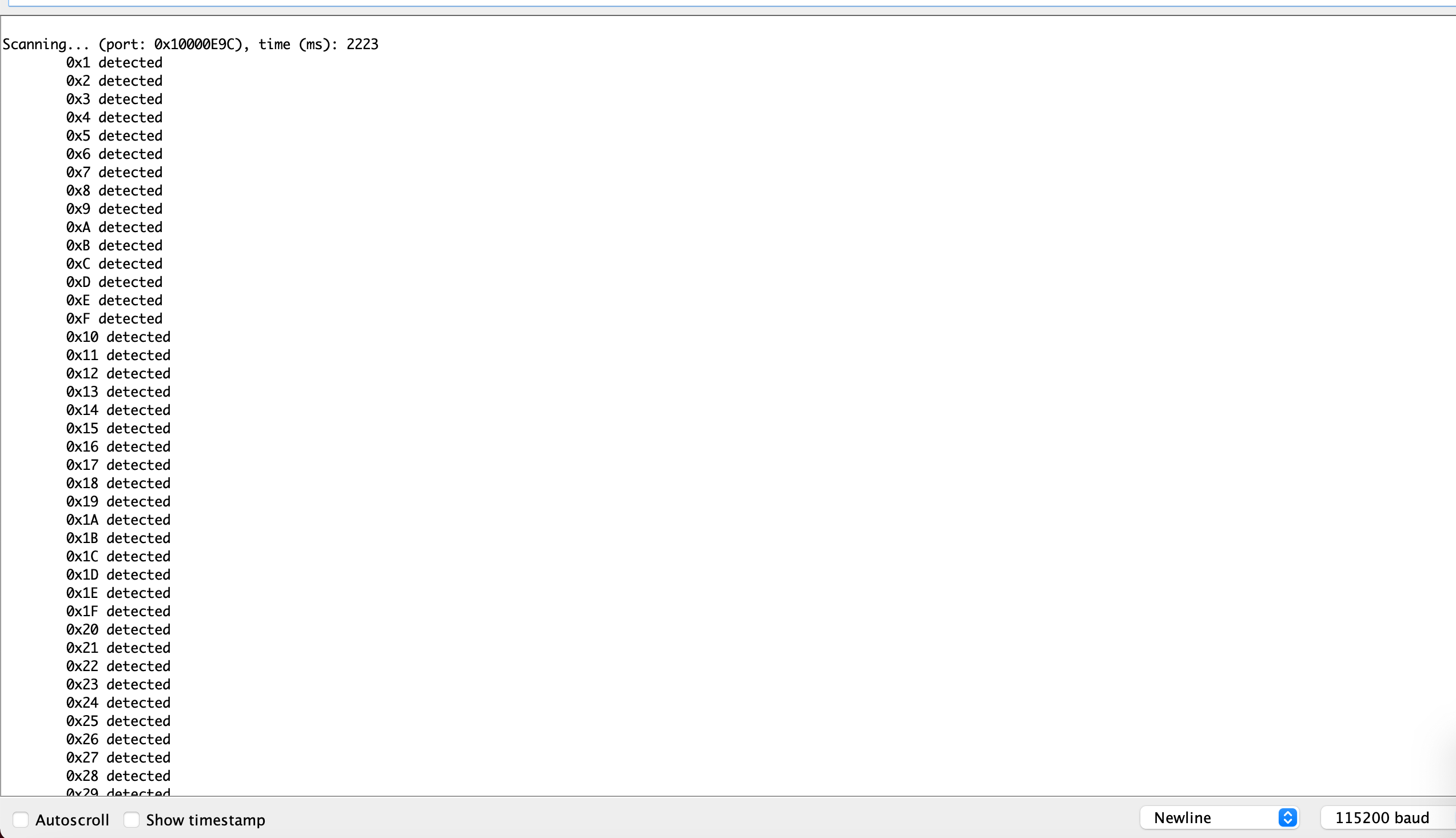
- I experienced the same common error when trying to read the I2C address of the time of flight sensor using the example script. The TA instructed me to paste a copy of my results showing the bug which was the common one experienced in the class.
- Looking at the data sheet shows that the benefit of using the short range mode on the time of flight sensor over the long range mode is “better ambient immunity”. This means that at shorter ranges, the sensor will be less sensitive to impoerfections and inconsistencies in the environment. The benefit of using the long range mode is obviously that you can see further and the drawback is that the sensor will have more error in certain environments. Because we are operating our cars in the fairly controlled enviroment of the lab, it will likely make sense to use the long range mode so that we can see further out. The medium mode obviously experiences both the pros and cons of each mode to a less extreme degree.
- To determine the ranging time of the sensor I utilized the millis() function which returns the number of milliseconds since the system was started. Since this value is always positive and can get quite big, I defined two unsigned long variables to store a start time and an end time. To determine the ranging time I set start time right before the sensor started ranging, and set end time right after the sensor actually got data. The ranging time was 3ms. Some pseudo-code and serial monitor results are shown below.
unsigned long startTime;
unsigned long endTime;
startTime=millis();
start sensor ranging;
///other stuff
sensor.getDistance;
endTime=millis();
sensor.clearInterupt;
sensor.stopRanging;
print endTime-startTime;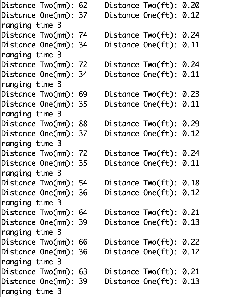
To measure reliability and repeatability of the sensor, I made some modifications to the code so that it would calculate the squared standard deviation of the first one hundred measurements that distance sensor one took and print it out to the screen. To do this I defined the following global variables.
//test reliability of the sensor
float reliability[100];
int times=0;
float total=0;
float sumOfs=0;
I then added the following to the loop function.
  //test reliability of the sensor
  if (times<100){
    reliability[times]=distanceOne;
    times+=1;
    total+=distanceOne;
  } else{
    int p;
    float average=total/100;
    for(p=0;p<100;p++){
      sumOfs+=(reliability[p]-average)*(reliability[p]-average);
    }
    Serial.print("standard deviation squared is ");
    Serial.println(sumOfs/100);
    delay(10000);
  }
I got the following at close range.
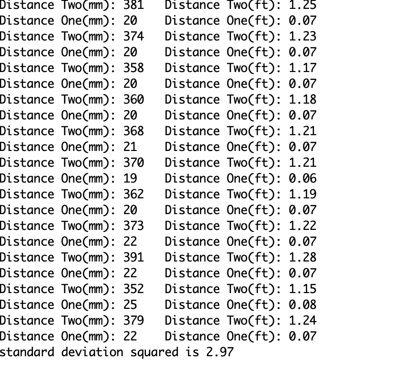
I got the following at a further range.
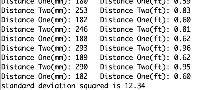
As we would intuitively expect the sensor seems to get less reliable at farther ranges.
Becuase the sensor is a ToF sensor it is not very sensitive to different colors or textures. I did however see some weird behavior on the sensor when I was measuring how far away it was from my computer screen. The values seemed to fluctuate more at a given distance and I am guessing it is because my computer screen is emitting light.
To measure the range of the sensors, I started at a wall and backed up until I started seeing unexpected sensor readings. The screenshot below demonstrated what this output looked like. Note the sensor in question is sensor 1. I saw the readings go up to about 2m and then after I backed up past that, the sensor readings started to decrease. I do not know if it was bouncing off of something other than the doorm, but this is the behavior I observed. In the screenshot I am backing up and you see it start to go up towards 2m and then begining to drop off after that.
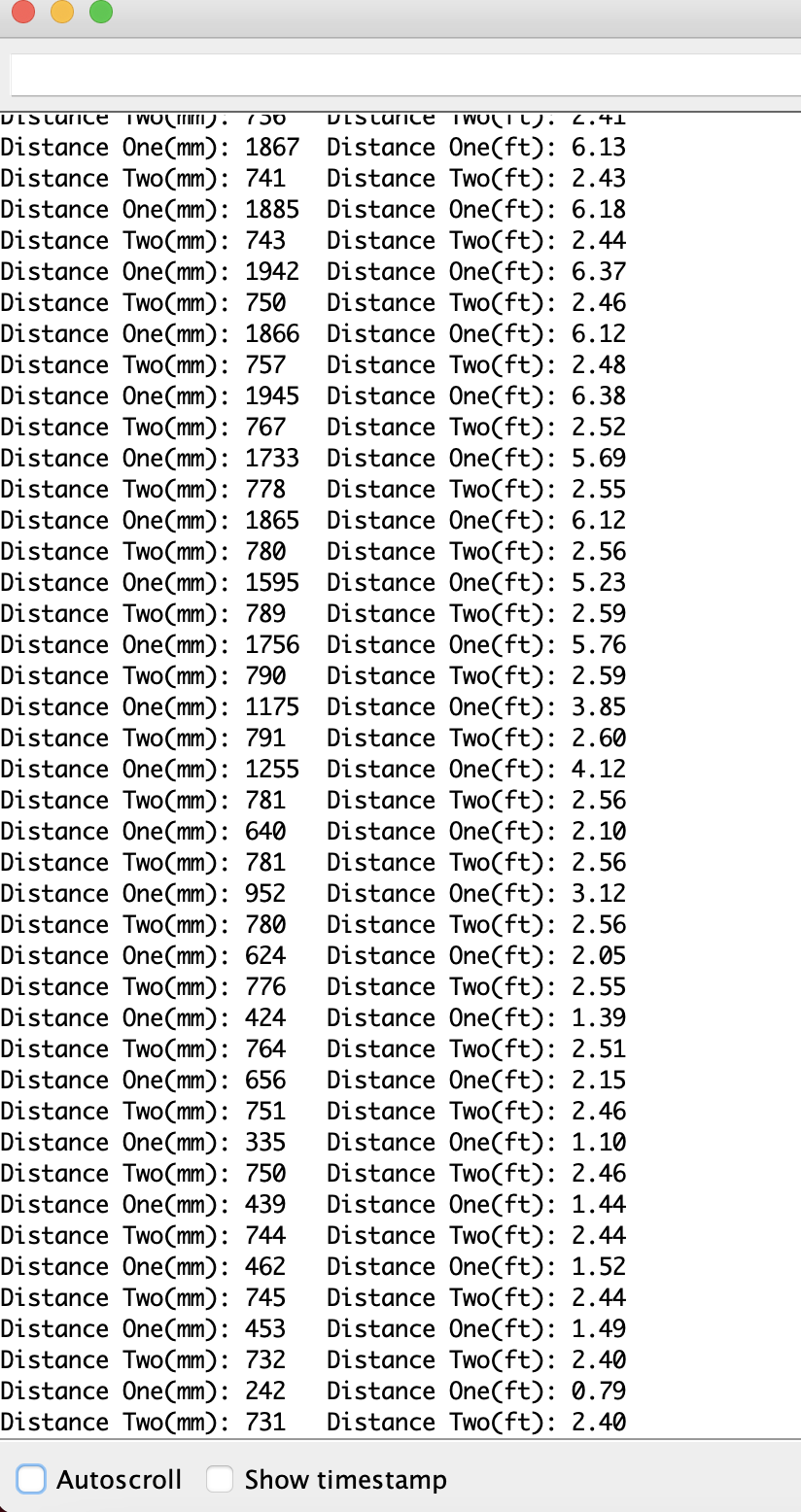
The sensor is fairly accurate, but the difference between actual value and measured value seems to increase as it is measuring object farther away.
The video below shows that I successfully hooked up and read from the 2 ToF sensors.
5690 Questions
- There are many types of IR sensors. 2 prevalent types are Amplitude based IR sensors and IR Time of Flight sensors. Amplitude based IR sensors work by having a transmitter send out infared light and then you have a receiver measure amplitude of the reflected light which will change with the distance that the light was reflected from. Time of Flight sensors also send out an infared signal and they measure the time it takes to see the reflection which gives you information about how far away the surface the light reflected off of is. These sensors do not technically measure the time between sending and receiving the signal, but instead they measure the phase difference between the sent signal and the reflected signal which is coorelated to the time.
Amplitude Based IR Sensors
Pros
- they are really cheap and have a small form factor
Cons
- affected by reflectivity of target
- does not work in settings with high amounts of ambient light
IR Time of Flight
Pros
- small form factor
- Not sensitive to target color, texture, or ambient light
Cons
- relatively expensive
- complicated processing
- they have a low sampling frequency (typically about 7-30Hz)
- they are really cheap and have a small form factor
- According to the documentation (https://cdn.sparkfun.com/assets/e/1/8/4/e/VL53L1X_API.pdf), the .setIntermeasurementPeriod(); function is used affects the sensor’s delay between two ranging operations. The .setTimingBudgetInMs(); function is the time that the sensor is allowed to perform one ranging operation.
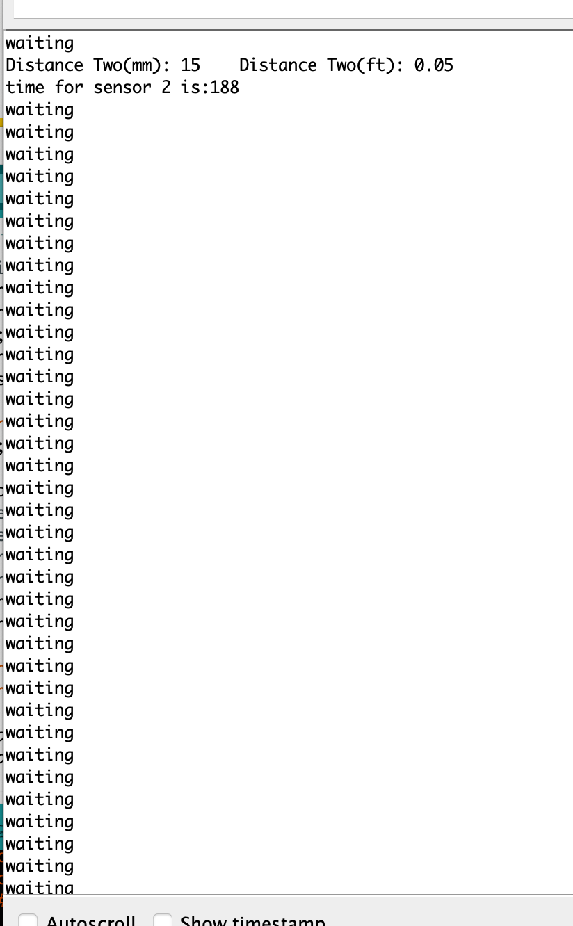
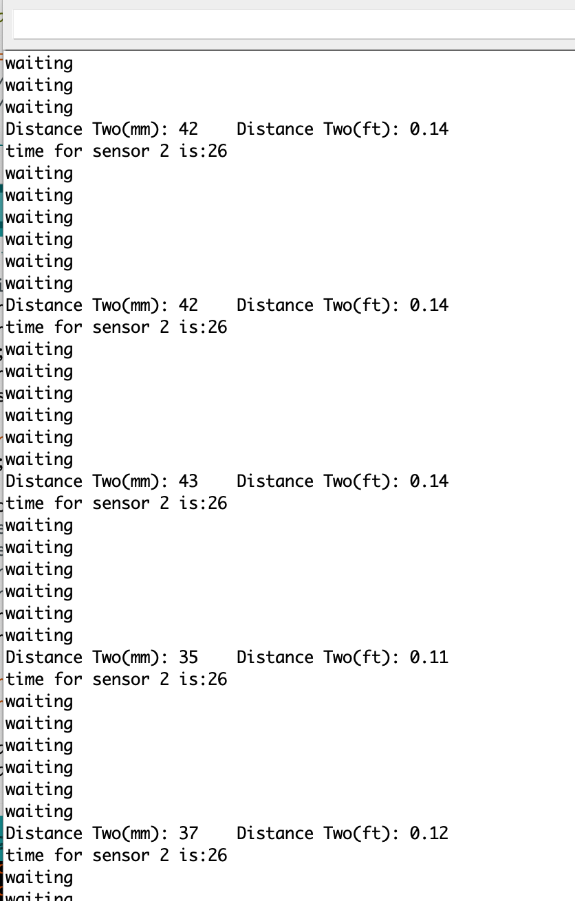
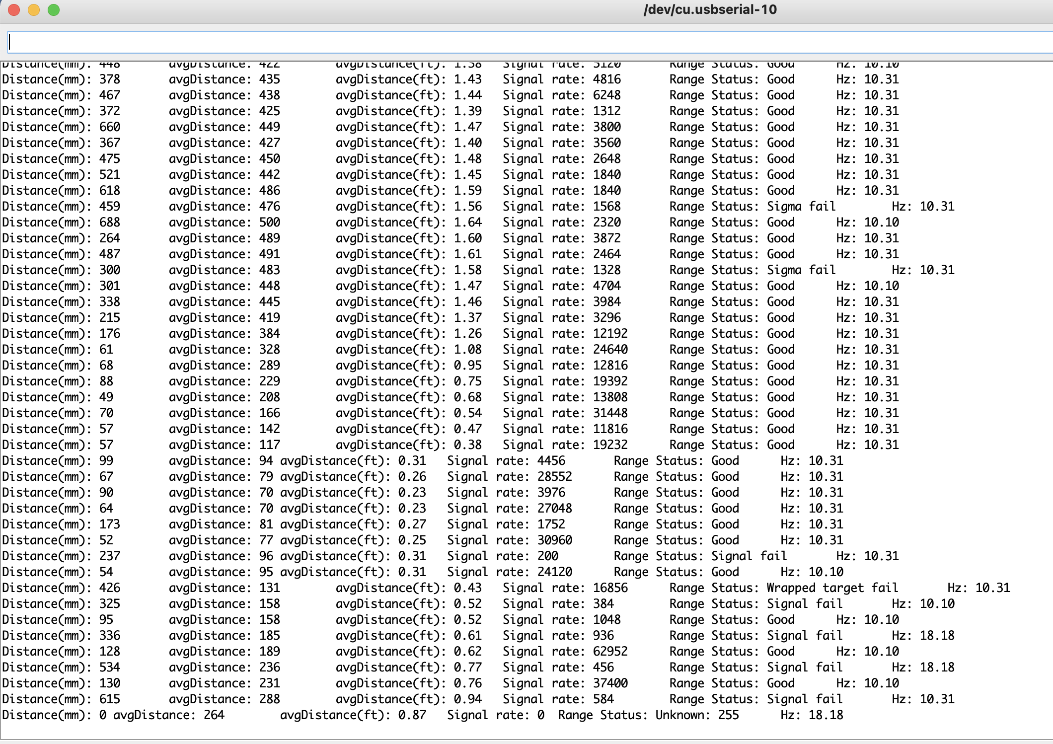
I used the millis to measure time. In this exercise, I just shutdown the first time of flight sensor. I then used the aformentioned functions on the second time of flight sensor. In one example I gave it a longer time to do what it needed to do setting the time budget to 200ms and the intermeasurement period to 800ms. This provided the results shown in the first screenshot below. I then put a heavier time constraint on the sensor by setting the time budget to 20ms and the intermeasurement period to 50ms. This sped up the sensor and provided the resutls shown in the second screeshot below. Given that the TOF sensor is fairly slow, it seems that as we are in a fast robotics course and we are not extremely power constrained, that we might want to decrease the intermeasurement period and try to ramp up our sampling rate.
slower
faster
- When I rapidly moved the sensor I received some measurements that were flagged as invalid. This is shown below. This might affect our robot when it is moving really fast. In future labs when we are dealing with measurements at high speeds, it might be wise to look at this signal and sigma and throw out measurements flagged as invalid.
part 3b IMU
-
I experienced the same common error when trying to read the I2C address of the time of flight sensor using the example script. The TA instructed me to paste a copy of my results showing the bug which was the common one experienced in the class.
-
IMU Setup: I ran the example script successfully as shown in the video below. The ADO_VAL represents the last bit of the IMU’s I2C address and should be 0. When I rotate the IMU about a given axis, move it, or flip it, I see a change in the 3 element arrays for the accelerometer and gyroscope as expected. I do not want to flip it around too much out of fear that my wiring will break.
Accelerometer
The video below shows my accelerometer being used to output roll and pitch. At this point the output has already been low passed using an alpha value of .2 which seemed to produce good results.
Below is the code I used to convert the accelerometer data into pitch and roll in terms of degrees.
float pitch_a;
float roll_a;
float LPF_p_a[2]={0,0};
float LPF_r_a[2]={0,0};
float alpha=0.2;
void loop()
{
  if (myICM.dataReady())
  {
    myICM.getAGMT();         // The values are only updated when you call 'getAGMT'
    pitch_a=180*atan2(myICM.accX(),myICM.accZ())/M_PI; //calculate and convert to degrees
    roll_a=180*atan2(myICM.accY(),myICM.accZ())/M_PI;
    LPF_p_a[1]=alpha*pitch_a+(1-alpha)*LPF_p_a[0];
    LPF_p_a[0]=LPF_p_a[1];
    Serial.print(LPF_p_a[1]);
    Serial.print(", ");
    LPF_r_a[1]=alpha*roll_a+(1-alpha)*LPF_r_a[0];
    LPF_r_a[0]=LPF_r_a[1];
    Serial.println(LPF_r_a[1]);

    delay(30);
  }
  else
  {
    SERIAL_PORT.println("Waiting for data");
    delay(500);
  }
}
Using the percent error equation of PE=100% * (actual-expected)/expected I examined the accuracy of the sensor at various positions. The results are below.
- When the sensor was held flat on the table (i.e. expected pitch and roll equal 0) pitch looked to be about 5 degrees off on average and roll looked to be about 1 degree off on avearge. However, there is no garuntee that my table is 100% perpendicular to gravitational pull either.
- At expected 90 degrees pitch was about 1 degree off (PE=1.1%) and roll was about 2 degrees off (PE=2.2%)
- At expected -90 degrees pitch was about 2 degrees off (PE=2.2%) and roll was about 2 degrees off (PE=2.2%) To measure these I tried to use the side of my computer and press the sensor as close to it as possible, but again it is not garunteed that the sides of my computer are perfectly aligned perpendiculary to gravitational pull.
Frequency Response
I followed this tutorial and altered it to fit my needs https://www.alphabold.com/fourier-transform-in-python-vibration-analysis/ I plotted an FFT of the roll measured by the accelerometer when I tapped it over 2 seconds. The FFT of the pitch would likely be similar. I added a delay of 5 seconds in the setup to give me some time to get ready to start tapping when data appeared on the serial monitor. I held the IMU flat on the table on as soon as I saw serial data, indicating that it had started to measure, I started tapping to simulate vibrations. Once 2 seconds had passed I put the system into an infinite while loop so that I could copy over the data. The Artemis code is summarize below.
int started=0;
long s;
void loop()
{
  if (started==0){
    s=millis();
    started=1;
  }
  if (millis()-s>=2000){
    while(1){
    }
  }
  //take IMU accelerometer data convert to role and print it to the console
  }
  delay(3)
}
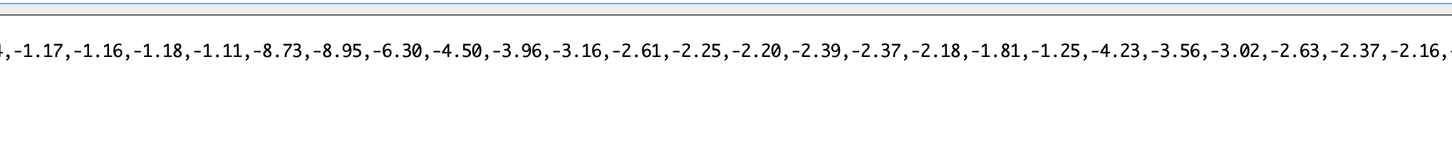
Here is what the console window looked like.
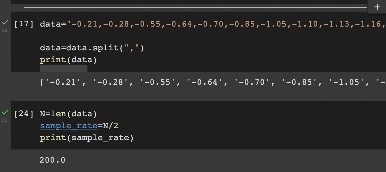
 I then used a control a to select all of the data and bring it over to the Python script and store it as a string. I then used the split function on the string to convert it into an array with all of the data. This also let me calculate how many samples I had taken and thus (with the assumption that all the samples were originally equally spaced apart in time) also the sampling frequency. A screenshot of this is shown below.
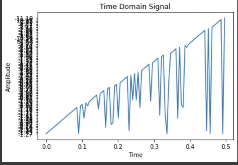
Once I had this, I plotted the output in the time domain and got something that looked like this.
I then did the following.
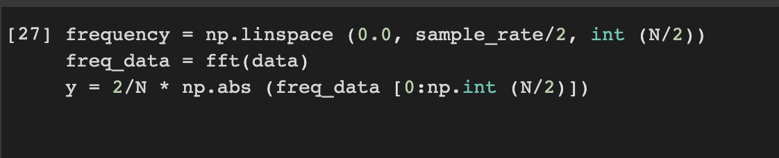
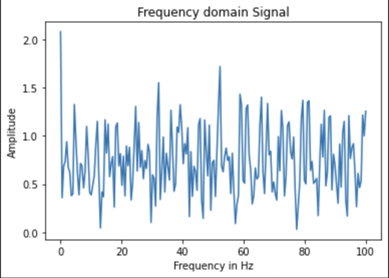
I used this information to plot the output in the frequency domain which is shown below.
I Then added the filter we saw in class which had an alpha of .2 and got the following in the time domain.
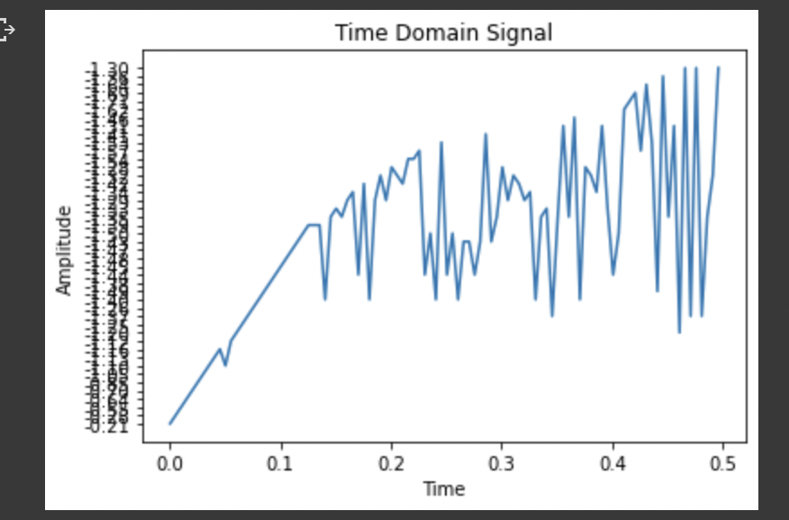
This corresponded to the following in the frequency domain.
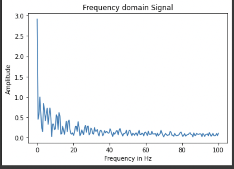
The more aggressive the cutoff frequency, the more you will supress noise, but the more your filtered output will lag the actual output of the sensor which is especially bad in fast robotics. Because of this you want to find a good balance between noise suppression and responsiveness and thus I will likely be playing around with the alpha parameter quite a bit throughout the semester.
Gyro
The video below shows that I completed the gyro portion and got the gyro working where I was computing roll, pitch, and yaw using the gyro.
The gyro is much less noisy than the accelerometer, especially when the accelerometer output is not filtered. However, when using the gyroscope to measure roll, pitch, and yaw, error accumulates and they drift away from the proper values. The accelerometer is much more accurate but the gyroscope is much less noisy. Becuase of this, combining the two sensors is a great way to utilize sensor fusion to achieve desirable results.
When dealing with the gyro, increasing the sampling frequency would likely cause error to accumulate faster, but it would also increase the resolution of the signal. Decreasing the sampling frequency would obvisouly have the opposite effect.
As mentioned previously the magnetometer and gyroscope outputs can be combined and used to produce a smooth and accurate output. This is a great example of sensor fusion. I used the code below to accomplish this.
float pitch_a;
float roll_a;
float alpha=0.1;
float pitch_g;
float roll_g;
float dt;
float last_time=0;
float pitch;
float roll;
void loop()
{
  dt=(micros()-last_time)/1000000.;
  last_time=micros();
  if (myICM.dataReady())
  {
//    Serial.println(myICM.gyrX());
    myICM.getAGMT();         // The values are only updated when you call 'getAGMT'
    pitch_a=180*atan2(myICM.accX(),myICM.accZ())/M_PI; //calculate and convert to degrees
    roll_a=180*atan2(myICM.accY(),myICM.accZ())/M_PI;
    pitch_g=pitch_g+myICM.gyrX()*dt;
    roll_g=roll_g+myICM.gyrY()*dt;
    pitch=pitch_g*(1-alpha)+pitch_a*alpha;
    roll=roll_g*(1-alpha)+roll_a*alpha;
    Serial.print(pitch);
    Serial.print(", ");
    Serial.println(roll);
    delay(30);
  }
  else
  {
    SERIAL_PORT.println("Waiting for data");
    delay(500);
  }
}
The video below shows the result. I will continue to play around with alpha to find the ideal balance as I meet new constraints in future labs.
5960 Extra Questions
I used the following code which was provided in the lab description to use the magnetometer to find true North.
  roll=roll_g*(1-alpha)+roll_a*alpha;
    pitch=pitch*M_PI/180; //convert back to radians
    roll=roll*M_PI/180;
    xm = myICM.magX()*cos(pitch) - myICM.magY()*sin(roll)*sin(pitch) + myICM.magZ()*cos(roll)*sin(pitch); //these were saying theta=pitch and roll=phi
    ym = myICM.magY()*cos(roll) + myICM.magZ()*sin(roll);
    yaw = atan2(ym, xm);
    Serial.println(yaw);
My results were not tremendously accurate. The video below shows this. In the video, the sensor reading does get fairly close to 0 as the sensor approaches true North as measured by my phone, and it clearly responds to changes in angle and thus could be useful later on.