Lab 11
In this report I will take you through my implementation of each of the steps of the Bayes filter and display the associated code.
Compute Control
def compute_control(cur_pose, prev_pose):
    """ Given the current and previous odometry poses, this function extracts
    the control information based on the odometry motion model.
    Args:
        cur_pose  ([Pose]): Current Pose
        prev_pose ([Pose]): Previous Pose
    Returns:
        [delta_rot_1]: Rotation 1  (degrees)
        [delta_trans]: Translation (meters)
        [delta_rot_2]: Rotation 2  (degrees)
    """
    delta_rot_1=np.degrees(np.arctan2(cur_pose[1]-prev_pose[1],cur_pose[0]-prev_pose[0]))-prev_pose[2]
    delta_trans=np.sqrt((cur_pose[1]-prev_pose[1])**2+(cur_pose[0]-prev_pose[0])**2)
    delta_rot_2=cur_pose[2]-prev_pose[2]-delta_rot_1

    return mapper.normalize_angle(delta_rot_1), delta_trans, mapper.normalize_angle(delta_rot_2)
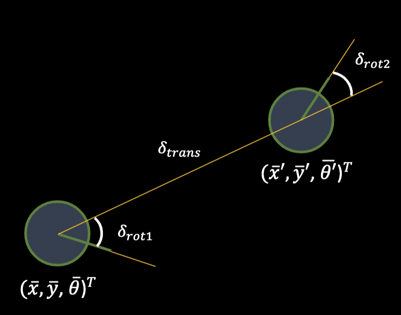
The compute control function essentially just tells you the control sequence necessary to take the robot from one pose to another. Every transition from one pose to another has 3 associated actions, the first rotation, a translation, and a second rotation. The figure below from the slides in class does a nice job of illustrating this.
The compute control takes in as arguments the robots current pose and the robots previous pose and returns the first rotation, the translation, and the second rotation that was used to take the robot from the previous pose to the current pose. Additionally, I normalize the angles which is important for making other steps of the Bayes filter work well when this function is used in the implementation of those steps.
Odometry Motion Model
def odom_motion_model(cur_pose, prev_pose, u):
    """ Odometry Motion Model
    Args:
        cur_pose  ([Pose]): Current Pose
        prev_pose ([Pose]): Previous Pose
        u=(rot1, trans, rot2) (float, float, float): A tuple with control data in the format
                                                   format (rot1, trans, rot2) with units (degrees, meters, degrees)
    Returns:
        prob [float]: Probability p(x'|x, u)
    """
    p1=loc.gaussian(mapper.normalize_angle(delta_rot_1_hat-mapper.normalize_angle(u[0])),0,loc.odom_rot_sigma)
    p2=loc.gaussian(delta_trans_hat,u[1],loc.odom_trans_sigma)
    p3=loc.gaussian(mapper.normalize_angle(delta_rot_2_hat-mapper.normalize_angle(u[2])),0,loc.odom_rot_sigma)

    prob=p1*p2*p3 ###probability for rotation 1 and translation and rotation 2

    return prob
The odometry motion model basically says, given what you think you did and where you think you were, what is the probability you are at a given place now. You break down the problem into the three actions involved with going from one pose to another (rotation 1, translation, rotation 2). You generate a gaussian with what you think you did based on your odometry sensors as the mean. The sigma of this gaussian, which relates to how spread out it is, depends on your sensors and is given to us in the code as loc.odom_rot_sigma for rotation and loc.odom_trans_sigma for translation. You also pass an ‘x’ to the gaussian function and the function inputs x to the function it generates and returns the output of the generated gaussian function given that input. You use the previously described compute control function to generate the “x’s” that you pass into the gaussian function. This essentially allows you to figure out step by step the probability that each one of the three actions did took you where you think it did. You then multiply all of these probabilities to figure out the probability that the total movement took you where you think it did.
Note in my code I often use x-mu as my ‘x’ input and 0 as the mu input to the gaussian which essentially just shifts the gaussian around 0 and has no effect on what I actually care about.
Prediction Step
def prediction_step(cur_odom, prev_odom):
    """ Prediction step of the Bayes Filter.
    Update the probabilities in loc.bel_bar based on loc.bel from the previous time step and the odometry motion model.
    Args:
        cur_odom  ([Pose]): Current Pose
        prev_odom ([Pose]): Previous Pose
    """
    mu=compute_control(cur_odom,prev_odom)
    loc.bel_bar=np.zeros((12,9,18))
    for xp in range(mapper.MAX_CELLS_X):
        for yp in range(mapper.MAX_CELLS_Y):
            for ap in range(mapper.MAX_CELLS_A):
                if loc.bel[xp,yp,ap]>0.0001: ###if the chance that I was in a state previously is sufficiently low ignore the calulations for that state
                    for xc in range(mapper.MAX_CELLS_X):
                        for yc in range(mapper.MAX_CELLS_Y):
                            for ac in range(mapper.MAX_CELLS_A):
                                cur_pose_c=mapper.from_map(xc,yc,ac) ###convert to continuous space from discrete map space before passing into motion model
                                prev_pose_c=mapper.from_map(xp,yp,ap)
                                loc.bel_bar[xc,yc,ac]+=odom_motion_model(cur_pose_c,prev_pose_c,mu)*loc.bel[xp,yp,ap]
    loc.bel_bar/=np.sum(loc.bel_bar) ### normalize
In the prediction step you go through every possible previous pose and every possible current pose. Because each state is defined by 3 states (x,y,angle) there are 6 nested for loops required to go through all of these states. Simply put, the prediction step says for every possible pose and every possible previous pose find the probabilty that I went from one pose to another pose and am in a given pose to begin with to find the probability that I am in any given state on the map now. In this you are updating the probabilities in loc.bel_bar (an array that represents the belief of the robot after the most recent prediction step) based on loc.bel (an array representing the belief of the robot after the most recent update step) from the previous time step and the odometry motion model.
The comments in my code do a decent job of explaining the subtleties of the implementation but I will expound a bit on them here. xp, yp, and ap are x previous, y previous, and angle previous respectivly. Similary, xc, yc, and ac stand for x current, y current, and angle current respectively. Thus I am saying with my iterations, for each of the previous states, go through all of the potential current states. Note the if statement in between the 3 loops for the previous state and the 3 loops for the current state. This if statement says that if there was a really low probability that I was in a state previously, don’t waste time doing the calculations to update bel_bar for the transitions involving these previous states because they will have little effect on the accuracy of bel_bar. This makes the code much more efficient and helps my simulation run much faster. In my code, the ‘c’ in cur_pose_c and prev_pose_c stands for continuous. The map is in discrete grid spaces and the from map function converts discrete pose information into continuous space so that it can be used by the odom_motion_model function. At the end I normalize (make all of the probabilties in bel_bar sum to 1) which is an important step in the Bayes filter.
Update Step
def update_step():
    """ Update step of the Bayes Filter.
    Update the probabilities in loc.bel based on loc.bel_bar and the sensor model.
    """
    ###update the belief that I am at any given cell based on my sensor measurements and my most recent prediction step
    for xc in range(mapper.MAX_CELLS_X):
        for yc in range(mapper.MAX_CELLS_Y):
            for ac in range(mapper.MAX_CELLS_A):
                loc.bel[xc,yc,ac]=loc.bel_bar[xc,yc,ac]
                for measurement in range(18):
                    #normalize(loc.gaussian(thsenosorvaluesIgot,thesensorvaluesishouldhaveseen,loc.sensor_sigma) times belief bar)
                    loc.bel[xc,yc,ac]*=loc.gaussian(loc.obs_range_data[measurement][0],mapper.get_views(xc,yc,ac [measurement],loc.sensor_sigma) ###multiply believed probability that I am in pose [xc,yc,ac] by the probability that I would see the sensor values I saw given I am at pose [xc,yc,ac] to update my believe probability that I am at pose [xc,yc,ac]
    loc.bel=loc.bel/np.sum(loc.bel)
In the update step, you are upating your loc.bel array based on the results of the prediction step you just ran, and your new sensor measurements that you just took. In the simulation, the update step generates a blue dot. In this step, I iterate through each of the possible poses that I am currently in. For each pose I look at the probability that I would get the sensor measurements that I got when I scanned given that I were in that pose and then multiply that by the probability that I were in that pose to begin with as calculated by my last prediction step. Because of this, I also iterate through each measurment in a given scan (it takes 18 measurements per scan). In this way I incorporate sensor measurements from my scan to get a better idea of the probability that I am in any given space on the map. I then also normalize which again ensures that all of the probablities sum to 1, an important step in the Bayes filter.
Result
Below is a video showing the result of my lab and that my Bayes filter worked well.
Debugging
One of the main things that made this lab challenging was narrowing down in which part of the code bugs were in. As demonstrated above, the functions that I was asked to implement oftne called each other and were intertwined. I found that looking at the simulator was helpful in identifying bugs during this lab. For example, I had a bug that took me a very long time to track down in my update step. However, the way that I eventually discovered was in my update step was noticing that the intial blue dot was off by much more than it should have been in the simulator. As I said before, the blue dot is generated by the update step. Thus when the initial blue dot was off by so much, I became much more confident that the bug lied in the update step and not the prediction step which seemingly had not even been run yet. Additionally, the update function did not even call odom_motion_model or computer motion control so I really suspected it was somewhere in update. Once I fixed that I was able to find another bug in my prediction step and eventually after enough bug fixes my simulation looked great!
Credits
I worked with Anya on a lot of this lab. Thank you to the TAs and to Professor Petersen for all there help in helping me wrap my head (at least partially) around the Bayes Filter!